
The Vlookup in Excel formula or formula is used to find the value of a lookup in a table. This formula is used to find the value in a range of cells containing a table which contains more than one column. The VLookup formula is VLookup(address, lookup_value, table_name, row_index_num, column_index_num, [lookup_type])
There are several ways to find answers to your Excel questions. Let us go through some of the more common ones and show you how to use Excel to find the answers you are looking for.
Vlookup is a useful formula in Excel that allows you to quickly find a value based on another value. For instance, you may need to quickly find a value based on a number of other values. Vlookup is very useful for quickly finding a value based on another value.
The greatest way to learn anything is to get your hands on it, make errors, and learn from them, as we all know.
As the saying goes, practice makes perfect.
That is the purpose of this Excel VLOOKUP Example tutorial.
A well-considered example, in my opinion, conveys an idea much better than an explanation of the underlying theory.
I carefully chose and described 10+ instances of the VLOOKUP function, rather than giving you a tedious study of every element of the VLOOKUP function.
These examples will show you how to utilize the function and how it may be used to a wide range of scenarios.
You’ll go through scenarios that address real-world issues while also expanding your Excel skills.
If you want to view the finest VLOOKUP examples, this tutorial is for you.
Don’t forget to save the sample file at the bottom of this page.
If you’re unfamiliar with the VLOOKUP function, I suggest reading these full VLOOKUP lessons for beginners before proceeding to the examples below. These examples will make more sense if you are familiar with the VLOOKUP syntax.
EXAMPLE 1 OF VLOOKUP: COMMISSION CALCULATOR
Workers in many sales positions are paid on a commission basis. Such employees’ commissions are often determined as a proportion of the sales they earned.
They get more commission and the business earns more money the more sales they make.
The commission may be set at a fixed fee, which is typically a percentage of any sales made by the representative, such as 7%.
Businesses may also employ progressive commission, in which the proportion of compensation increases when sales representatives meet specific goals.
For example, if a salesperson sells $10,000 worth of products or services, he or she will get a 10% commission on the first $10,000, a 15% commission on the following $10,000, and so on.
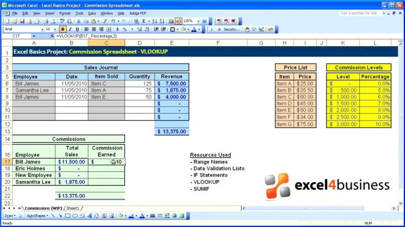
The worksheet below demonstrates how to use the VLOOKUP function to calculate a sales rep’s commission depending on how much money she earns.
“Range lookup” is the name of this VLOOKUP sample. This indicates that the algorithm is searching for a match that falls within a range of values rather than an exact match (approximate match).
For example, as seen in the table above, the VLOOKUP formula returned 5% for any value below 20,000, 8% for any value between 20,000 and 30,000, and so on.
Analysis of the VLOOKUP Formula
Let’s take a closer look at the formula utilized in the last case.
=VLOOKUP(F4,Commision Schedule,2,TRUE)
In fact, the image says it all.
In the equation;
- The first parameter pointed to the cell containing the value to be searched for. (Cell F4 is the one I’m referring about.)
- The second argument also refers to the table from which the commission rate is calculated. (This is the table Commision Schedule.) A named range or a regular range may be used as the table array parameter. The range B4:C14, for example, is the same as the commision Schedule. If you insist on using a regular range rather than a named range, make it an absolute reference, such as $B$4:$C$14.
- The third parameter indicates the table column from which the commission rate should be calculated. (This is the second column in the lookup table.)
- The last parameter is TRUE, which stands for “approximate match.” The biggest value that is smaller than the lookup value will be found using VLOOKUP approximate match. For example, in the example above, the formula in cell G4 looked up $46,356 in the lookup table’s first column. Because the database didn’t find an exact match for this search, the commission rate for the greatest amount less than the lookup value (which is $40,000) was obtained.
You may use the fill handle to copy the formula to the rest of the cells after you’ve completed writing the formula in the first cell.
EXAMPLE 2 OF VLOOKUP: INCOME TAX RATE CALCULATOR
If you are familiar with accounting, this example will make more sense to you (Taxation to be precise). You are free to skip to the next example if you despise accounting.
We’ll create a formula that returns the tax rate for different income levels in this VLOOKUP example.
Another excellent option for the VLOOKUP function in Excel is a tax rate calculator (range lookup to be specific).
In accounting, there is a tax system known as the progressive system of taxation, in which the income of people and businesses is taxed at a rate that increases over time.
This implies that the greater your income, the higher your tax percentage, and the smaller your income, the lower your tax percentage.
In fact, if you make very little money, you will not have to pay any income tax.
It’s known as Tax Brackets, and it’s the division in which tax rates vary when taxable income rises or falls.
The following tax table summed it up perfectly:
The following schedule exemplifies the progressive tax system well.
As you can see, low-income workers earning less than $5,000 are not required to pay any taxes on their earnings.
You are only eligible for tax after your income reaches $5,000 or more, although you will pay a low tax rate as a beginning.
Each cent or dollar you make moves you into a different tax bracket or category, resulting in a higher tax rate when your taxable income moves into a new bracket or category.
The aim of this Excel VLOOKUP example now is to create a formula that will return the tax rate for every given salary.
The lookup table is B6:D13 in the preceding spreadsheet, and the lookup value is in column G6, which contains the taxable income.
The salary amount in cell G6 is nowhere to be found in the first column of the lookup table, thus if this formula was searching for an exact match, it would have encountered an error.
However, in this instance, the algorithm does a range lookup, which means it is searching for a match that falls inside a certain range of numbers — in this example, between $80,000 and $104,000.
It returned the tax rate for the salary category as soon as it discovered it.
Remember that the formula only looks at the first column of the lookup table to get the tax rate base, not the first two columns. The second, or center, column serves as a reference point for understanding the different tax rates and categories.
Let’s have a look at the analysis now.
Analysis of the VLOOKUP Formula
The formula utilized to complete the job in this case is as follows:
=VLOOKUP(G6,B6:D13,3)
- This formula’s first parameter refers to the cell containing the taxable income we’re searching for. (Cell G6 is the name of the cell.)
- The second argument also refers to the table from which the tax rate is calculated. (It’s cell B6:D13.)
- The third parameter indicates the table column from which the tax rate should be calculated. (This is the third column in the lookup table.)
But hold on! VLOOKUP has four parameters, however this formula only utilizes three of them and yet produces no errors.
This is because when dealing with a “range lookup,” the final parameter is optional (approximate match).
VLOOKUP uses an approximate match by default. As a result, if you leave out the final parameter, VLOOKUP will infer that you accept the approximate match as the default match.
However, if you wish to always include the match type, set this argument to TRUE or 1.
If the number you’re searching for isn’t in the lookup column, Excel won’t give you the usual #N/A error notice if you use the approximate match. Instead, the greatest value that is less than the given number will be used.
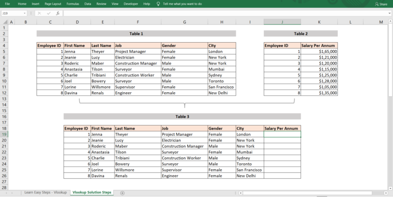
EXAMPLE 3: Using ID, return goods and prices.
Have you used any excellent accounting software before?
If you answered yes, you already know how simple it is to create invoices.
The goods, as well as their pricing, are completely integrated and presented in an appealing manner.
When you input a product ID, the name and price for that product appear without you having to type them in.
The VLOOKUP feature in Excel may also be used to create such a system.
Both the product and price columns in this example have two versions of the VLOOKUP function.
The amount column, on the other hand, does not have a VLOOKUP formula. To obtain the total amount, it simply multiplies the quantity by the price.
As a result, our aim is to create two formulae that will return the product name and price when a product ID is given.
Keep in mind that in the previous two instances, we used the approximate match to do ranging lookups. In this case, though, we want to discover precise matches for our search keywords. As a result, this is a VLOOKUP example that is an exact match.
The worksheet above is set to display formulas. Excel shows formulae instead of the results in this mode.
Let’s take a realistic look at the two formulae in the next section.
Example 3 of Analysis of the VLOOKUP Formula
The lookup table in the products column is B4:D14, which has been renamed to ProductList, and the lookup value argument refers to the matching cells in the ID column, which hold the product ID, as seen in the worksheet.
The lookup table in the invoice’s price column is B4:D14, which similarly uses the named range (ProductList), and the lookup value argument refers to the matching cells in the Id column, which provides the product ID.
The column index parameter, which is the column from which the formula gets a value, is the sole variation between these two formulae.
- Both of the above formulae’ initial arguments relate to the same cell, which includes the product ID we’re searching for. (Cell G6 is the name of the cell.)
- The second and third parameters both relate to the same product list database, from which the product name and price are extracted. (ProductList has been renamed to cell B4:D14.)
- The third parameter specifies the table columns from which the product name and price should be retrieved. (Column 2 has the product name, and column 3 contains the price.) The only formula that changes between the two VLOOKUP formulae is this one.
- The match type is the fourth parameter. The FALSE match type is used in both formulae, indicating that a precise match is required.
This is an exact lookup, not a range lookup, as previously stated.
As a consequence, if a product ID isn’t found in the lookup table, the formula will return an error, as opposed to the approximate match, which uses the highest value that is smaller than the lookup value.
Because the product ID cannot be located in the products list table, errors occur in all of these fields.
How do you deal with mistakes like this?
This job qualifies to be used as an example. Let’s go on to the next step.
EXAMPLE 4: VLOOKUP in the event of a mistake
One of the reasons VLOOKUP isn’t functioning is because Excel can’t locate the value you’re searching for, as you can see in the following example.
This is the most frequent reason. However, this is not always the case. Sometimes the reason is so enigmatic that you don’t know where to start looking.
True, the VLOOKUP function is strong, but it isn’t without flaws. It has side effects, just as most wonderful things.
This VLOOKUP example will teach you why VLOOKUP value mistakes happen and how to avoid them.
You should be aware that a VLOOKUP value error occurs when the lookup value is not found in the first column of the lookup table.
Let’s look at how to deal with the #N/A issue using the worksheet from VLOOKUP example 3.
The source of the mistake is obvious in this spreadsheet.
The product IDs (15, 16 and 17) associated with the error cells are clearly missing from the lookup database (or product list table).
If the goods in question are new to your list and need to be included, the apparent remedy to the value issue is to add them to the product list.
To do so, just add three rows to the products list table and add the product IDs, names, and pricing to the database.
The invoice template works properly without problems after you add the missing items to the product listings.
If you need to add missing records to the lookup table, this method is a necessity. What if you don’t have to?
If Excel can’t locate the search phrase, you may want it to do nothing or something different.
You can have Excel place a blank value in the cell instead of the irritating #N/A error message, or return a nicer message like a hyphen (-).
In the example above, the formula does not encounter any errors when you input a product that does not exist in the products list database, unlike previously when the #N/A error appeared.
The solution to this issue is to utilize conditional logic to determine whether or not a product ID is accessible. This method is known as IF ERROR VLOOKUP by some.
The method used in this case is called =IFERROR().
First and foremost, it examines the formula to determine whether the results are correct. If an error occurs, this method will not perform VLOOKUP. If there are no errors, it will just execute the lookup formula.
The IF ERROR VLOOKUP formulae for the two columns are shown below:
In the product column, type
=IFERROR(VLOOKUP(G5,ProductList,2,FALSE),”-“)
If you use relative cell references for the first argument, the formula in the first cell may be duplicated into each cell in the product column (which is the lookup value)
Regarding the pricing column,
=IFERROR(VLOOKUP(G5,ProductList,3,FALSE),”-“)
The identical formula in the first cell may be duplicated into each cell in the price column utilizing relative cell referencing for the lookup value, much like the product column.
The worksheet shown above is in display formula mode, which enables you to view all of the worksheet formulae rather just the final numbers.
The IFERROR function in this formula has a straightforward purpose: it checks to see whether the VLOOKUP will produce any errors. Excel executes the VLOOKUP smoothly if the formula does not encounter any errors. If there is a genuine mistake, though, a hyphen is returned instead of #N/A.
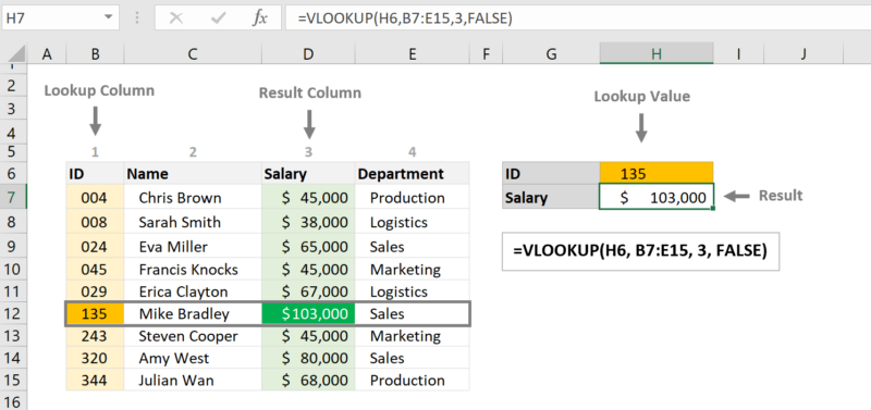
EXAMPLE 5: Calculating a student’s grade
If you’re a student, a teacher, or have ever been one of these two, the concept in this example and the following two will make greater sense to you.
A list of students’ names is included in the table below, along with their test results in different courses.
Assume you wish to get David’s math score back.
The table is divided into five columns, with the names column on the left and the scores of different courses in the remaining four.
The goal is to create a VLOOKUP formula that searches the names column for David and returns his Math score.
VLOOKUP Formula Analysis
VLOOKUP FORMULA FACTS: When dealing with a range lookup, when an approximate match is required, you can only disregard the final parameter. When the parameter is not provided, an approximate match is used by default. However, if you’re using VLOOKUP to get an exact match, be sure to include this parameter or you’ll receive bad results.
Let’s look at how the formula got David’s Math score in its most basic form.
To begin, it looks for the name David in the first column (or leftmost column) in the lookup table.
When it finds the name in the list, it counts to the right until it reaches the fourth column (the Math column), where it retrieves the score from the cell that corresponds to the name David.
VLOOKUP FORMULA FACTS: By default, VLOOKUP can only search the lookup table’s leftmost column. VLOOKUP, for example, will fail if you pick a table and wish to look in the second or third column. Always bring the lookup column first when preparing your data for VLOOKUP to prevent problems.
Any student’s score for any course may be retrieved using the same method.
It’s as simple as altering the column index number: 2 retrieves the English score for the given student, 3 retrieves the French score, 4 retrieves the Match score, and 5 retrieves the Science score for the particular student.
For instance, the formula below will provide Khan’s French score:
=VLOOKUP(G4,A1:E12,3,0)
The number of the column index has been altered from four to three. The algorithm will get Khan’s French score since French is in the third column and the lookup value in cell G4 is Khan.
To update a student’s name, just modify the value in the cell where the lookup value is stored, which is cell G4.
If you alter cell G4 to any student’s name in the list, the algorithm will automatically adapt the result to that student’s French score.
However, this worksheet has a restriction.
You can only alter the student’s name in cell G4 to get his result; however, you must update the formula to the appropriate column number to change his score for a different course.
What if the worksheet user could get a score by selecting the student name as well as the course name without having to modify the formula again?
It’s worth elaborating on this point. Continue to the following example to discover this technique.
EXAMPLE 6 OF VLOOKUP: TWO-WAY LOOKUP
Double lookup is another name for two-way lookup.
It’s a formula that searches in both vertical and horizontal directions at the same time to locate a cell where two columns and rows meet.
This request may be handled in two ways: one using VLOOKUP + MATCH and the other using INDEX+MATCH.
Unless you use a helper function, which happens to be the MATCH function, the VLOOKUP function cannot perform this job on its own.
The match function’s aim in this case is to return the index number of the course we selected in the worksheet.
To demonstrate, let’s make a few changes to the worksheet from the prior example.
Take a look at what we’ve got with a bit more work.
The student exam score table is on the left, and a small dashboard on the right of the table enables the spreadsheet user to choose a student name and course to get results depending on the chosen parameters.
The MATCH formula presented here makes the formula so flexible that it automatically adjusts the column from which to get the score when the user changes the course.
Analysis of the VLOOKUP formula
The formula for a two-way lookup is as follows:
=VLOOKUP(G4,A1:E12,MATCH(H4,A2:E2,0),FALSE)
Like the previous instances, this formula contains four parameters. The only difference is that it takes another function (col index num) as its third parameter.
The MATCH function in the formula is utilized to provide our VLOOKUP a number, which the VLOOKUP then utilizes as its third parameter (col index num).
If you call the MATCH function by itself, it will return a number reflecting the location of the course you choose (AKA column number).
=MATCH(H4,A2:E2,0)
The match function utilized the course name in cell H4 as the lookup value and returned its location in range A2:E2 as seen below (the second row of the table).
When you enter Math in cell H4, the formula returns 4, indicating that the Math scores are in the fourth column.
You may use the VLOOKUP formula to search the whole range of cells for the right score thanks to the Match function.
To make it more interesting, you may choose the student’s name and classes from a drop-down list rather than putting them in manually.
In the following example, we’ll look at how to use this approach.
VLOOKUP with drop-down List (EXAMPLE 7)
To modify the search keywords (the name and the course) in the previous example, you’ll have to manually put them in, but you may just as simply use an In-Cell drop-down list.
Manually entering data increases the likelihood of inputting incorrect data into a formula’s input field. “Trash in, garbage out,” the coders will remark.
And, as a spreadsheet user, you should be aware that Excel formulae are only as good as the data that they are given.
As a result, you or someone else using your spreadsheet may use this VLOOKUP method to enter the student name and course without having to type them in manually.
This is what I’m attempting to convey in the image below:
The formula used in the previous example remained unchanged in this case.
All you have to do now is build a drop-down list for the cells that hold the lookup values (cell G6 and H6).
To learn how to make an Excel drop down list, follow these steps:
- Click to activate the cell (Cell G6 and H6) for which you want to create a list: Because we require two lists for two different cells, you’ll have to make them one by one.
- Go to Data / Data Tools / Data Validation / Data Validation / Data Validation / Data Validation / Data Valid Go to the Data Tools category under the Data tab and choose Data Validation.
- Three tabs show in the Data Validation dialog. Allow is a “validation criterion” under the settings tab; click the drop-down box below it and choose list.
- Select the range that includes the list in the box underneath the Source criterion. (For the names, use =$A$3:$A$12, and for the courses, use =$B$2:$E$2).
You’ll be able to put in the student’s name and courses without having to type them in manually after completing these procedures for both cells.
VLOOKUP FROM ANOTHER SHEET (EXAMPLE 8)
You’ll learn how to use the VLOOKUP formula to get a value from a separate sheet in this example.
It’s not always the case that your VLOOKUP table and the actual formula are on the same worksheet.
The table you’ll need to search up and get data is sometimes in a separate worksheet.
Take, for example, the following Excel invoice template. When you download and view the sample file, you’ll see that one page (named the pricing sheet) contains a product catalog, while the following sheet (called the invoice sheet) constructs the invoice.
The invoice worksheet, in this case, must utilize formulae that relate to data from the preceding sheet, which contains the product catalog.
This is a worksheet with a very simple invoice template. We have a comparable invoice in VLOOKUP example 3 that gets items and prices from a separate database but in the same worksheet.
However, in this template, I’m going to show you how to bring a template like this to life by utilizing the VLOOKUP function to extract product prices from a separate sheet.
If you haven’t already, you should download the sample file to learn more about the VLOOKUP example with many sheets.
Look in this example workbook for another worksheet called PriceList, which is located immediately below the example 8 worksheet.
A table with two columns – goods and price – is included on this page.
In this example, we’ll create a formula that conducts a VLOOKUP from another sheet, obtaining the prices of items in the price column from another sheet.
The formula for doing a VLOOKUP between two sheets is as follows:
=VLOOKUP(C17,PriceSheet!B2:C18,2,FALSE)
Analysis of the VLOOKUP formula
Let’s dissect this formula and figure out what’s actually going on.
- C17: The lookup value is stored in this cell.
- PriceSheet!B2:C18: This is the lookup table from another sheet. To get the product price, the formula uses a table from another page. This method is simple: in the second parameter of the function, just precede the range or table name with the worksheet name, followed by an exclamation mark, to perform VLOOKUP from another sheet.
- 2: This is the table column number from which the product price will be retrieved. The number 2 in this parameter refers to the lookup table’s second column, which is the price column.
- FALSE: This implies that the formula should return a result that is an exact match for the value in cell C17’s lookup field.
You may utilize the drop-down list method in the previous example for the product column if you want your worksheet to have additional functionality.
This manner, you or your spreadsheet user can rapidly load your invoice with items while the VLOOKUP formula gets their pricing with only a few mouse clicks..
VLOOKUP FROM ANOTHER WORKBOOK (EXAMPLE 9)
VLOOKUP is often performed from another worksheet in the same spreadsheet.
VLOOKUP from another worksheet, on the other hand, is less frequent.
The possible issue with this kind of connection is that the linked worksheet may or may not always be accessible.
The connection is broken if you rename or transfer the referenced workbook to a new place.
Excel, on the other hand, being as clever as it is, does not leave you totally stuck in this scenario. Instead, it keeps working with the most current version of the data it could get before the connection went down. You’re in luck!
You’ll learn how to use the VLOOKUP formula to get a value from a separate workbook in this example.
It’s not always the case that your VLOOKUP table is in the same workbook as your VLOOKUP table, as in the preceding example.
In certain cases, the table where you’ll search for and obtain data will be in a different workbook.
The idea to apply here is almost identical to that of the prior case.
When providing the [table array] parameter, insert the workbook name at the beginning of the reference and then surround it in square brackets to execute VLOOKUP from another workbook. The sheet name, an exclamation mark, and the range address or name come after the file name.
Download the sample file and open it in a new Excel worksheet on your PC if you truly want to understand how this works.
Leave the default file name and worksheet name as Book1 (for the file name) and sheet1 (for the worksheet name) (for the sheet name).
If you’re going to use a separate workbook for this example, call it Book1 and make sure it includes a sheet1 worksheet.
You are welcome to bring your own workbook and worksheet titles if you are familiar with this material and are certain that you will not be confused. It will work nicely if you use the appropriate methods.
Now that you have everything you need, open the newly created workbook and build a product catalog in the sheet1 worksheet, just as in the previous example.
If you like, you may copy and paste the table. Ensure, however, that you begin copying or constructing your table in cell A1.
Return to the example 9 worksheet and enter the following formula in the price column:
=VLOOKUP(C17,[Book1.xlsm]Sheet1! $A$1:$B$17,2,0)
The lookup value in the formula is C17, which refers to the material in Cell C7. You will get an error if you enter any product name in this column.
The product price will be retrieved using this VLOOKUP function from the desktop worksheet Book1.
If you wish to VLOOKUP from another workbook, all you have to do is put the name of the workbook in square brackets, then the sheet name, an exclamation mark, then the range.
If you don’t want to manually input the [table array] parameter, you may use a simple trick to have Excel do it for you.
To begin, open the workbook you wish to reference. Book1 on the desktop in our instance.
Next, when you’re ready to provide the [table array] parameter in the formula, use Alt+Tab to go to Book1, then pick the product catalog table or range.
Look in the address bar to see that Excel has already done the referencing for you; now input the remaining parameters and hit enter to run the function.
EXAMPLE 10 OF VLOOKUP: Partial text match using wildcard
Your data’s content may sometimes be so complex that you don’t know precisely what you’re searching for.
Consider the following data: the client names in the customer column are prefixed with their account numbers.
How would you look for a client in this scenario if you just have the names of the customers?
What you actually need in these situations is a search tool that is flexible enough to keep an eye out for results that are close but not identical.
Excel’s wildcard characters make it easy to search for any portion of a cell’s content, which will please power searchers.
For example, in the table above, you may search for a client just by his name without having to bother about account numbers.
In Excel, there are three wildcards for advanced lookups. However, in this case, we’ll use the most common one, the asterisk (*) wildcard.
The link below will take you to a comprehensive guide on the subject.
VLOOKUP wildcard – a step-by-step tutorial is a related link.
Let’s suppose you want to get the profit on a client called Harper using the table above, but you don’t have the number that goes with his name.
Let’s examine what happens if we do a regular VLOOKUP without the wildcard using the following formula.
=VLOOKUP(D3,B5:F18,5,FALSE)
Do you see what I mean?
The algorithm attempted to locate a client named Harper in order to recover the profit your business earned with him.
Despite the fact that you have an employee with that name, the data indicates that the name does not exist.
Excel is a pretty straightforward individual, therefore you must be similarly straightforward while interacting with him.
Instead than simply looking for Harper, try searching for Harper* using the asterisk wildcard.
Yes, you read it correctly. Add an asterisk to the name you want to search for.
This is how the formula should now look:
=VLOOKUP(“Harper*”,B5:F18,5,FALSE)
Do you want to know what went wrong?
That’s all there is to it.
In the calculation, the asterisk wildcard is used to substitute all of the digits following the customer name – Harper.
Similarly, if you want to search on the most recent numbers, just replace Harper with the asterisk wildcard (*550318), and Excel will locate the column based solely on the numbers.
To summarize, if you wish to search for starting characters, place them before the asterisk (*). Bring those characters following the asterisk (*) if you’re looking for concluding characters.
The lookup values (customer name/number) are hard-coded in this example, but the asterisk wildcard may also be used to get information from other fields.
Concatenate the cell address with an asterisk (*), for example, if the customer name is in another cell, and Excel will happily run your formula with the wildcard.
The following formula used the value in cell D3 as the lookup value and use the concatenate sign (&) to append the asterisk (*) wildcard.
=VLOOKUP(D3&”*”,B5:F18,5,FALSE)
Oh! I nearly forgot about it.
To save time typing, you may alternatively utilize a dropdown list of the names.
Refer to example 7 for additional details on utilizing an excel drop down list in VLOOKUP.
VLOOKUP MULTIPLE CRITERIA EXAMPLE 11
If two conditions are fulfilled, you may need to use VLOOKUP in certain situations.
This is unfortunately one of the three most frequent VLOOKUP flaws.
Excel is set up in such a manner that it can only search through one column for a matching value when the search phrase is discovered.
Does this rule out the possibility of utilizing the VLOOKUP function to search up a value using multiple criteria?
That is far from the case.
You may run VLOOKUP with as many criteria as your data allows using the method described in this example.
From January through April, this spreadsheet displays the monetary amount of sales produced by sales reps.
Assume you want to know how much money Alexa earns in March.
Alexa occurs four times in the table’s leftmost column. If you search for Alexa using the VLOOKUP function, the formula will find the first instance of Alexa in the list.
Your goal, though, is to find the fourth Alexa appearance, which correlates to the March sales figure.
You may utilize the helper column method to get around the function’s shortcoming.
This method allows you to concatenate the two columns into a new column, then look at the combined column instead.
The combined column is now a helpful column for you in this instance.
You may use the helper column as a lookup column to get any employee’s sales number for any month after combining the two columns in the helper column.
For example, if you want to discover Alexa’s sales for March, use the lookup value “Alexa|March.”
The formula is as follows:
=VLOOKUP (“Alexa|March”,D6:E25,2,FALSE)
Conclusion
Congratulations! You’ve made it all the way to this stage!
You may now proclaim yourself a VLOOKUP ninja by shouting at the top of your lungs. It is, without a doubt, a significant achievement.
You not only learned how to use the VLOOKUP function, but you also acquired a few Excel tricks and methods that are well worth your time.
More in-depth Excel lessons like this one may be found on this site.
Excel is a great tool for solving business problems, but it can be even better depending on how you use it. Just because it’s a spreadsheet doesn’t mean you have to use it that way. Excel has a variety of powerful functions that are designed to solve business problems. The VLOOKUP function is one of the most commonly used functions in Excel, but it’s also one that I’ve seen some people misuse.. Read more about how to do vlookup in excel with two spreadsheets and let us know what you think.
Frequently Asked Questions
How do you do a VLOOKUP step by step?
To do a VLOOKUP, you must first find the column that contains the value you are looking for. In this case, we want to find the Age column in the Employee table.
How will you use VLOOKUP () in Excel answer with example?
VLOOKUP () is a function in Excel that allows you to look up values in a range of cells. It can be used with text, numbers, or formulas. If you are looking for the value in column A and the value in column B, then type =VLOOKUP(B1,A1).
What is VLOOKUP in Excel with example?
VLOOKUP is a function in Excel that allows you to find information from one table and put it into another. For example, if you have a list of names and want to know what their email addresses are, you can use the VLOOKUP function with the email address column as the lookup value.


