
In this article, we will focus on one of the most useful functions in Excel, the MATCH function. The MATCH function is a conditional function that returns the smallest value that meets a given criterion. In this article, we will look at how to use the MATCH function in Excel as well as some of the properties of the MATCH function.
Excel’s MATCH function is a powerful tool that can be used to do a lot of things. However, it is not commonly used by most Excel users. So, in this post, I will show you some of the steps that you should take to use the MATCH function in your Excel workbook. ~
In this tutorial we will learn how to use MATCH Function in Excel. Let’s learn how to use MATCH Function in Excel with examples.
What is Excel’s MATCH function?
The MATCH function is used to find a value in a range and find the location of a cell that matches the search phrase.
If you have a list of names in a column, this function may search through those names to find the position of a certain name you provided.
This is one of those functions that is less helpful until it is used in combination with another function. Lookups are frequently performed using it and the INDEX function.
Syntax of the MATCH function
=MATCH(lookup value, lookup array, [match type]) =MATCH(lookup value, lookup array, [match type]) =MATCH(lookup_
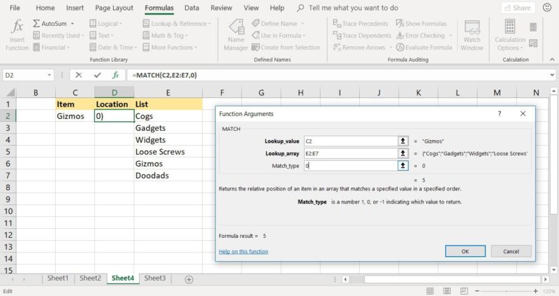
The lookup value, the lookup array, and the [match type] are the three parameters to this function.
Let me briefly clarify these reasons before I take you through an example. When dealing with real-life instances, it will help you comprehend them better.
- lookup value: The value you’re searching for is represented by this parameter. Excel will provide a number that reflects the value’s location when it finds it. It’s possible that this value be text or numbers.
- lookup array: The range you wish to search across is represented by this parameter. The range must be one-dimensional when providing the lookup array. This implies you can only look for information in a particular column or row. You may, for example, search through A1:A10 or A1:G1. You can’t, however, search a grid of cells (like A1:G10 which include several rows and columns).
- [match type]: This parameter specifies the method for finding a match. With a match type of zero, the location of the first item that matches precisely is returned. The 0 match type is utilized in the majority of instances. So, until you know what you’re doing, I strongly advise you to stick to it. With a match type of 1, the location of the biggest value that is equal to or less than the searched value will be returned. With a match type of -1, you’ll get the location of the lowest value that’s equal to or larger than the value you’re looking for.
What is the MATCH function and how do I write it?
Bring your equal symbol first, followed by the term match.
Let me demonstrate this method to you. Excel will display you all the functions that begin with the letter M if you start entering the function with the first letter M.
Fortunately, the MATCH function is the first recommended function. As a result, there is no need to write everything out. Simply hit the tab key, and Excel will automatically enter the function.
(lookup value) is the first parameter of the match function.
Now provide the lookup value, which is the function’s first parameter.
Because we want to find David’s position in the list, the lookup value will be “David.”
Always enclose the lookup value with double quotes if it is the text, as in David. In the case of numbers, however, there is no need for quotation marks.
You may also utilize the content of another cell as the lookup value by making a reference to it. If you select B2 as your lookup value, for example, the content of cell B2 will be utilized as the lookup value.
This also implies that if you alter the content in cell B2, you’ll change the lookup value, and the match function’s result will change as well.
(lookup array) is the second parameter of the match function.
Let’s go on to the second parameter, the lookup array, now that we’ve specified the first.
The range in which Excel will search for our lookup value is specified by this parameter (which is David).
As I previously said, the lookup array must be one-dimensional when creating this method. This means you can only search one row or column at a time. However, searching across a grid of cells with many columns and rows is impossible.
We’ll have to look at cells A5 through A14 since we’re searching for the name David. As a result, A5:A14 will be the lookup array.
Match the third argument of the function ([match-type])
Now we’ll look at the following parameter, the [match type].
There are three kinds of matches here.
Excel will retrieve the location of the biggest value that is equal to or less than the lookup value if the match type is 1 (one).
Larger than is represented by a match type of -1, which will return the location of the lowest value that is equal to or greater than the lookup value.
When looking for numbers, these two kinds of matches make sense. When you don’t know the precise value you’re searching for, it comes in useful. Excel will provide a result based on the value that is closest to the search phrase.
When working with text, however, always use a match type of 0.
Exact match is indicated by a match type of zero: this match type will return the location of the first item that matches precisely.
The 0 match type is utilized in the majority of instances. So, until you know what you’re doing, I strongly advise you to stick to it.
Close the parenthesis and press enter to execute the formula now that all of the parameters have been exhausted.
Result
The outcome is 5, indicating that David is in position number five. David is, in other words, the fifth name on the list.
If there is no match – in other words, if David isn’t in the list – the function will return a #N/A error, indicating that the item you’re searching for isn’t in the database.
This is how the MATCH function works.
What you need to know about the MATCH function
- The MATCH function is unaffected by case. This implies that DAVID and David are the same person (or David).
- Only one-dimensional arrays are supported by the MATCH function (range). This implies you can only look at cells in the same column or row at a time. The function will return #N/A if your lookup array contains a range with a grid of cells that includes many rows and columns.
- In the event of a match type of zero, the MATCH function returns #N/A if no match is discovered. However, the method may return an approximate match for match types 1 and -1.
- If you’re using a MATCH type of 1 or -1, make sure the range’s data is ordered in ascending order.
- When the MATCH type is zero and the search phrase is text, you may conduct a partial search by using wildcard characters.
Conclusion
By alone, the MATCH function does not seem to be very helpful. When coupled with other tasks, though, it becomes very useful.
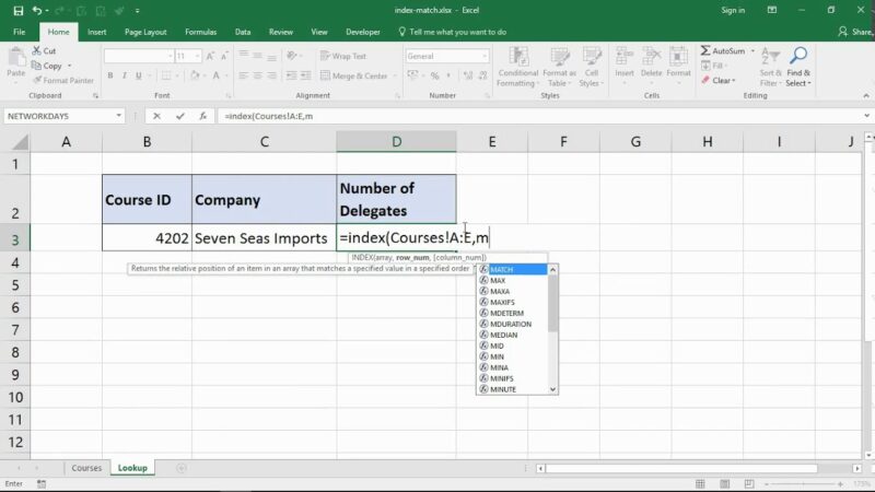
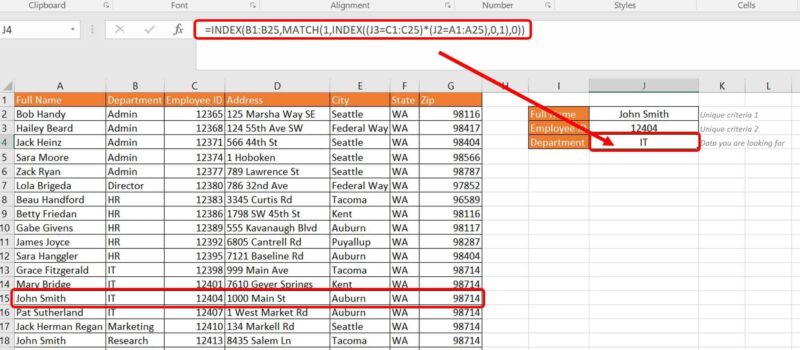
The following articles show how the MATCH function may be used with another function (INDEX):
How to use INDEX-MATCH to do a double lookup
How to use INDEX-MATCH to do a left lookup
The MATCH function in Excel is a powerful tool which you can use to find and choose a given set of records from a database table, based on a certain criteria. It can be used in multiple ways, such as to find a record that matches a certain criterion and appears at least X number of times. This article provides a tutorial to learn the basics of the MATCH function and how to use it to find records in a database table, based on a certain criteria.. Read more about how many options are available in the match type parameter of the match function in ms excel and let us know what you think.
Frequently Asked Questions
What is a match function in Excel?
A match function in Excel is a formula that returns the value of one cell if it is equal to another cell.
How do I compare 2 columns in Excel?
To compare 2 columns in Excel, you can use the following formula: =VLOOKUP(A1,B1,2)
How do you match similar text in Excel?
If you want to match similar text in Excel, you can use the Find and Replace function.


